bidser

CRAN

BIDS dataset reading and navigation tools

Installinstall.packages('bidser')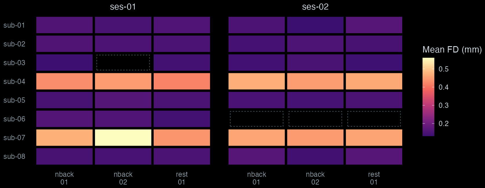

Grid of subjects by session and run, each cell coloured by the run's mean framewise displacement; subjects 04 and 07 are bright across all runs, and four dashed cells mark missing runs

Mean framewise displacement of every BOLD run in a simulated two-session study, read with read_confounds() and arranged by the entities query_files() parsed from the file names. Dashed cells are runs missing from the dataset.

Project bids_project() over raw data and derivatives/ pipelines

Queries query_files() by subject, session, task, run and other entities

Tables Events, fMRIPrep confounds, JSON sidecars with inheritance

Testing create_mock_bids() writes small stub datasets

What it does

A dataset becomes one object

bids_project() reads a BIDS directory and returns a bids_project object that records every file with the entities parsed from its name. By default it requires participants.tsv, discovers pipelines under derivatives/, and caches a file index in .bidser_index.rds at the dataset root, which it rebuilds when the directory’s modification time changes.

The dataset here was written by create_mock_bids(), which builds a stub dataset from a table of files. It writes participants.tsv and dataset_description.json with their contents; every other file is zero-byte. Rows marked fmriprep = TRUE go under derivatives/fmriprep/, which gets its own dataset_description.json, so bids_project() opens the stub without warnings. Here the BOLD and confound files are empty; features 03 and 04 write event and confound tables into the same tree and read it again.

The simulated dataset has 8 subjects and 44 BOLD runs; 4 of the 48 subject-by-run cells in the figure are missing.

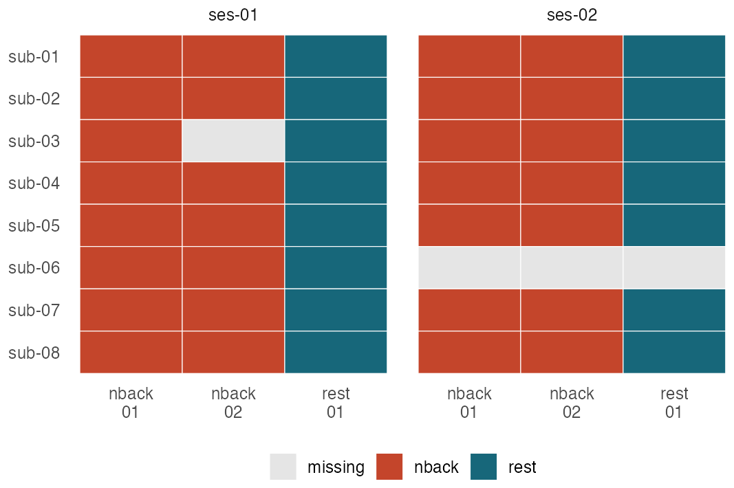
Grid of eight subjects by two sessions of three runs each, n-back runs in coral and rest runs in teal; sub-03's second session-1 n-back run and all of sub-06's session 2 are grey for missing

Simulated dataset. Each cell is one BOLD file returned by query_files().

library(bidser); library(dplyr)
library(tidyr); library(ggplot2)
set.seed(7)

# Simulated study: 8 subjects x 2 sessions, two n-back runs
# and one rest run per session. Sub-06 missed session 2;
# sub-03 lost an n-back run.
runs <- expand_grid(subid = sprintf("%02d", 1:8),
                    session = c("01", "02"),
                    task = c("nback", "nback", "rest")) |>
  mutate(run = sprintf("%02d", row_number()),
         .by = c(subid, session, task)) |>
  filter(!(subid == "06" & session == "02"),
         !(subid == "03" & session == "01" & run == "02"))

# Write a BIDS tree of zero-byte BOLD files and fMRIPrep
# confound files, and read it
root <- tempfile("study-")
files <- bind_rows(
  mutate(runs, suffix = "bold.nii.gz", fmriprep = FALSE),
  mutate(runs, suffix = "desc-confounds_timeseries.tsv",
         fmriprep = TRUE))
create_mock_bids("nback-study", sprintf("%02d", 1:8),
  mutate(files, datatype = "func"),
  create_stub = TRUE, stub_path = root)
proj <- bids_project(root)

# One row per BOLD file, with its parsed entities
bold <- query_files(proj, regex = "_bold\\.nii\\.gz$",
                    return = "tibble")
grid <- mutate(bold, cell = paste0(task, "\n", run)) |>
  complete(subid, session, cell)

tile_plot <- function(d, fill, values) {
  ggplot(d, aes(cell, paste0("sub-", subid))) +
    geom_tile(aes(fill = {{ fill }}), colour = "white") +
    facet_grid(~ paste0("ses-", session)) +
    scale_fill_manual(values = values) +
    scale_y_discrete(limits = rev) +
    labs(x = NULL, y = NULL, fill = NULL) +
    theme_minimal(base_size = 13) +
    theme(panel.grid = element_blank(),
          legend.position = "bottom")
}
fig <- tile_plot(grid, coalesce(task, "missing"),
                 c(nback = "#c4452b", rest = "#17677a",
                   missing = "grey90"))

Files selected by their BIDS entities

query_files() selects files by entity (subid, session, task, run and others) and by a regular expression on the file name. It returns paths relative to the dataset root, or, with return = "tibble", one row per file with its parsed entities, sorted by subject, session, task, run and path.

Entity values are regular expressions matched anywhere in the label, so subid = "0" matches all eight subjects here. match_mode = "exact" requires the whole label to match, and match_mode = "glob" takes shell-style wildcards.

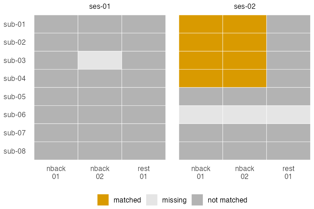
The query returns 8 of the 44 BOLD files. Each row also carries the file’s scope (raw or derivatives), pipeline, extension, datatype, size and modification time.

The same subject-by-run grid with the eight session-2 n-back runs of subjects 01 to 04 in amber, other runs in grey, and missing runs in light grey

file	subid	run
`sub-01_ses-02_task-nback_run-01_bold.nii.gz`	01	01
`sub-01_ses-02_task-nback_run-02_bold.nii.gz`	01	02
`sub-02_ses-02_task-nback_run-01_bold.nii.gz`	02	01
`sub-02_ses-02_task-nback_run-02_bold.nii.gz`	02	02
`sub-03_ses-02_task-nback_run-01_bold.nii.gz`	03	01
`sub-03_ses-02_task-nback_run-02_bold.nii.gz`	03	02
`sub-04_ses-02_task-nback_run-01_bold.nii.gz`	04	01
`sub-04_ses-02_task-nback_run-02_bold.nii.gz`	04	02

The rows returned by the query, which are the amber cells in the figure; all have session 02 and task nback.

# Session-2 n-back runs for subjects 01-04. Entity values
# are unanchored regular expressions unless match_mode
# says otherwise.
hits <- query_files(proj, regex = "_bold\\.nii\\.gz$",
                    subid = "0[1-4]", session = "02",
                    task = "nback", return = "tibble")
hits |> select(file, subid, session, task, run)

grid <- left_join(grid, mutate(hits, hit = "matched") |>
                    select(subid, session, task, run, hit),
                  by = c("subid", "session", "task", "run"))
fig <- tile_plot(grid, case_when(is.na(path) ~ "missing",
                                 is.na(hit) ~ "not matched",
                                 .default = hit),
                 c(matched = "#d99a00",
                   `not matched` = "grey70",
                   missing = "grey90"))

Event files from every run in one table

read_events() reads each events.tsv that matches its subject, session, task and run patterns and returns a nested tibble with one row per file: the entities in .subid, .session, .task and .run, and the event table in data. It also returns undotted copies of the entities (task, session, run, participant_id), and the tibble is grouped by run, so it is ungrouped before tidyr::unnest().

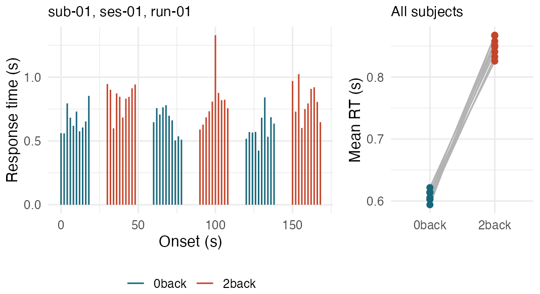
Here it has 29 rows, one per n-back run, holding 1,740 trials in all. The nested tables keep every column of the TSV (onset, duration, trial_type, response_time) and add .file, the path it was read from.

Unnested, it becomes one trial table for the whole study, from which the figure plots a single run and the per-subject means.

Left: response time of each trial in one n-back run plotted at its onset, 0-back blocks in teal and 2-back blocks in coral. Right: each subject's mean response time, higher for 2-back than 0-back in all eight subjects

.subid	.session	.task	.run	data
01	01	nback	01	tibble, 60 × 5
01	01	nback	02	tibble, 60 × 5
01	02	nback	01	tibble, 60 × 5
01	02	nback	02	tibble, 60 × 5

Simulated events: response times drawn from log-normal distributions, slower for 2-back trials. The table shows the four rows of the nested tibble for sub-01.

# Simulated events.tsv for each n-back run: six blocks of
# ten trials, alternating 0-back and 2-back
bids_file <- function(r, suffix, dir = root) with(r,
  file.path(dir, sprintf("sub-%s/ses-%s/func", subid,
                         session),
  sprintf("sub-%s_ses-%s_task-%s_run-%s_%s",
          subid, session, task, run, suffix)))
nb  <- filter(runs, task == "nback")
blk <- rep(0:5, each = 10)
for (i in seq_len(nrow(nb))) readr::write_tsv(tibble(
  onset = blk * 30 + rep(0:9, 6) * 2, duration = 0.5,
  trial_type = c("0back", "2back")[blk %% 2 + 1],
  response_time = rlnorm(60, -0.5 + 0.3 * blk %% 2, 0.2)
), bids_file(nb[i, ], "events.tsv"))

# Re-read the tree, then read every n-back event file:
# one row per run, with the event table nested in `data`
proj <- bids_project(root)
ev <- read_events(proj, task = "nback")
trials <- ev |> ungroup() |> unnest(data)

library(patchwork)
one_run <- filter(trials, .subid == "01", .session == "01",
                  .run == "01")
p1 <- ggplot(one_run, aes(onset, response_time,
                          colour = trial_type)) +
  geom_segment(aes(xend = onset, yend = 0)) +
  labs(x = "Onset (s)", y = "Response time (s)",
       colour = NULL, title = "sub-01, ses-01, run-01")
p2 <- trials |>
  summarise(rt = mean(response_time),
            .by = c(.subid, trial_type)) |>
  ggplot(aes(trial_type, rt, group = .subid)) +
  geom_line(colour = "grey70") +
  geom_point(aes(colour = trial_type), size = 2) +
  labs(x = NULL, y = "Mean RT (s)", title = "All subjects") +
  guides(colour = "none")

fig <- (p1 + p2 + plot_layout(widths = c(2, 1))) &
  scale_colour_manual(values = c(`0back` = "#17677a",
                                 `2back` = "#c4452b")) &
  theme_minimal(base_size = 13) &
  theme(legend.position = "bottom",
        plot.title = element_text(size = 12))

Sidecar metadata and confounds for each run

get_metadata() returns the JSON metadata that applies to one file under BIDS inheritance, merging sidecars from the least to the most specific location. read_confounds() reads fMRIPrep confounds tables from derivatives/; confound_set() names standard groups of columns, such as "fd", "motion6", "36p" and "acompcor", and matches them across the column names used by different fMRIPrep releases.

For sub-01_ses-02_task-nback_run-01_bold.nii.gz, get_metadata() returns RepetitionTime = 2 s, inherited from the task-level sidecar task-nback_bold.json at the dataset root; with provenance = TRUE it also lists that file as the source. In the simulated confounds of the 29 n-back runs, framewise displacement exceeds 0.5 mm in 36% (sub-04) and 41% (sub-07) of volumes; in every other subject the share is below 2%.

variables_table() combines the scans, events and confounds of each run into one row with nested tables.

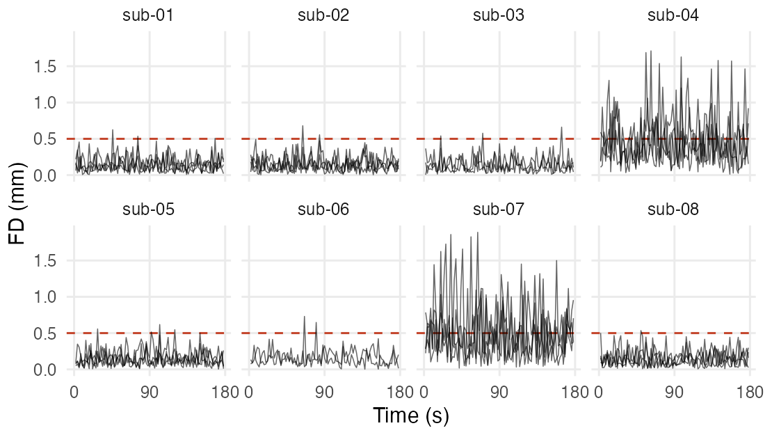
Eight panels, one per subject, of framewise displacement over the 180 s run for each n-back run, with a dashed line at 0.5 mm; sub-04 and sub-07 often exceed it, the others rarely

Simulated framewise displacement. The dashed line marks 0.5 mm; time uses the RepetitionTime resolved from the sidecar.

# Fill each run's confound file with simulated framewise
# displacement over 90 volumes; sub-04 and sub-07 move more
prep <- file.path(root, "derivatives", "fmriprep")
for (i in seq_len(nrow(runs))) {
  f <- bids_file(runs[i, ], "desc-confounds_timeseries.tsv",
                 dir = prep)
  m <- if (runs$subid[i] %in% c("04", "07")) 0.45 else 0.15
  readr::write_tsv(tibble(framewise_displacement =
    c(NA, rgamma(89, 2, 2 / m))), f, na = "n/a")
}

# A task-level sidecar at the dataset root applies to every
# n-back run; more specific sidecars override its keys
jsonlite::write_json(
  list(RepetitionTime = 2, TaskName = "n-back"),
  file.path(root, "task-nback_bold.json"), auto_unbox = TRUE)
proj <- bids_project(root)
md <- get_metadata(proj, hits$path[1], provenance = TRUE)
tr <- md$metadata$RepetitionTime     # seconds

fd <- read_confounds(proj, task = "nback",
                     cvars = confound_set("fd"),
                     nest = FALSE) |>
  mutate(time = (row_number() - 1) * tr,
         .by = c(participant_id, session, run))

fig <- ggplot(fd, aes(time, framewise_displacement,
                      group = interaction(session, run))) +
  geom_hline(yintercept = 0.5, linetype = "dashed",
             colour = "#c4452b") +
  geom_line(linewidth = 0.3, alpha = 0.6, na.rm = TRUE) +
  facet_wrap(~ paste0("sub-", participant_id), nrow = 2) +
  scale_x_continuous(breaks = c(0, 90, 180)) +
  labs(x = "Time (s)", y = "FD (mm)") +
  theme_minimal(base_size = 13) +
  theme(panel.grid.minor = element_blank())

Development version

The install command above gives the CRAN release. To install the development version from GitHub:

pak::pak("bbuchsbaum/bidser")

Every figure on this page is drawn by software/showcase/bidser/make-figures.R in the site’s source, and the code shown with each figure is the code that drew it.