fmrihrf
CRANHemodynamic response functions, basis sets and event regressors for fMRI
install.packages('fmrihrf')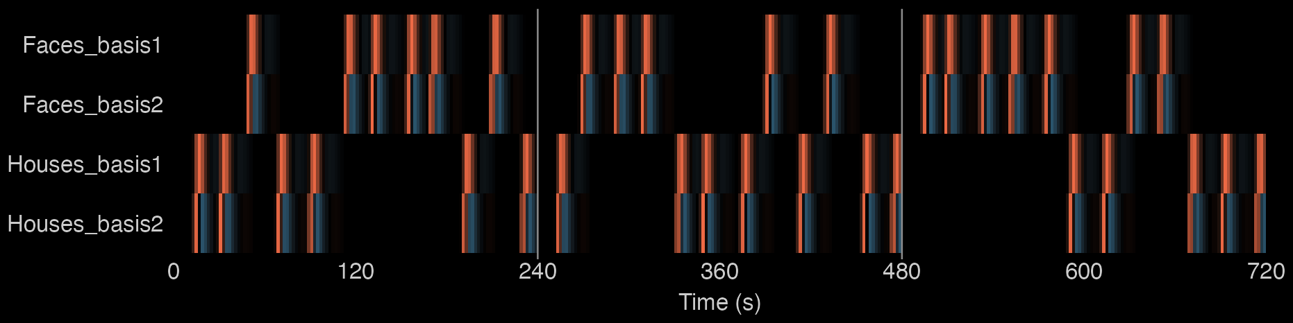
The design matrix for three simulated runs, built by regressor_design() with HRF_SPMG2; section 04 shows the code.
HRF shapes SPM canonical and derivatives, gamma, Gaussian, half-cosine, boxcar
Basis sets FIR, B-spline, tent, Fourier, Daguerre, libraries over a parameter grid
Regressors Onsets, durations and amplitudes, convolved with the HRF in C++
Timing Sampling frames, run-relative onsets, multi-run design matrices
What it does
01
An HRF is a function of time
HRF_SPMG1, HRF_GAMMA, HRF_GAUSSIAN and the other predefined HRF objects are R functions: called with a vector of times in seconds, they return the response at those times. Each object also records its span and its number of basis functions. gen_hrf() turns a shape function such as hrf_half_cosine() into an HRF object and can add a lag, an event width and normalization. block_hrf() convolves an HRF with a boxcar width seconds long to model a sustained event.
HRF_SPMG1 peaks at 5.0 s with a value of 0.175 and reaches its undershoot minimum (-0.016) at 15.8 s. With summate = TRUE, the default, the response to a 12 s event peaks 5.4 times higher than the response to a brief event.
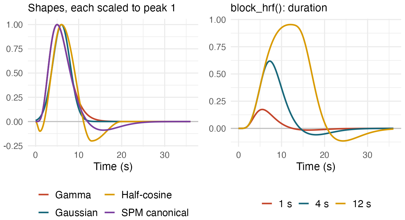
Left: each curve scaled to a peak of 1 by evaluate(normalize = TRUE); the half-cosine has f1 = -0.1 (initial dip) and f2 = -0.2 (undershoot). Right: unscaled.
library(fmrihrf)

# An HRF object is a function of time in seconds
HRF_SPMG1(c(0, 5, 16))  # onset, peak, undershoot

shapes <- list(
  "Gamma"         = HRF_GAMMA,
  "Gaussian"      = HRF_GAUSSIAN,
  "Half-cosine"   = gen_hrf(hrf_half_cosine,
                            f1 = -0.1, f2 = -0.2),
  "SPM canonical" = HRF_SPMG1
)
# Sustained events: the canonical HRF convolved with
# a boxcar of the given width in seconds
blocks <- list(
  "1 s"  = block_hrf(HRF_SPMG1, width = 1),
  "4 s"  = block_hrf(HRF_SPMG1, width = 4),
  "12 s" = block_hrf(HRF_SPMG1, width = 12)
)

t <- seq(0, 36, by = 0.1)
fig <- draw(curves(shapes, t, normalize = TRUE),
            "Shapes, each scaled to peak 1") +
  draw(curves(blocks, t), "block_hrf(): duration",
       ncol_legend = 3)
02
A basis set lets a GLM estimate the response shape as well as its amplitude
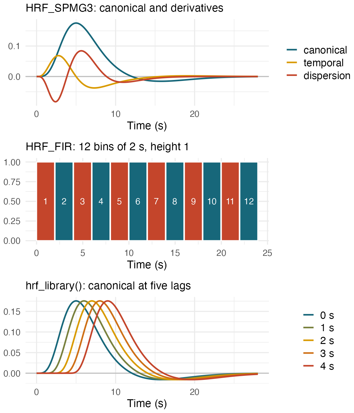
A basis set is an HRF object with more than one basis function. evaluate() returns a matrix with one column per function, and a regressor built from the set contributes one design-matrix column per function. HRF_SPMG3 is the SPM canonical HRF with its temporal and dispersion derivatives; HRF_FIR divides the 24 s after an event into 12 bins of 2 s. hrf_library() builds a basis by calling a generating function once for each row of a parameter grid, here the canonical HRF at lags of 0 to 4 s. Generators such as hrf_fir_generator() and hrf_fourier_generator() set the number of functions and the span.
# A basis set is an HRF with several columns; a GLM
# fits one coefficient per column
lib <- hrf_library(function(lag) lag_hrf(HRF_SPMG1, lag),
                   data.frame(lag = 0:4))
sapply(list(HRF_SPMG3, HRF_FIR, lib), nbasis)  # 3 12 5

# evaluate() returns a time x basis-function matrix
tb <- seq(0, 28, by = 0.05)
fig <- draw_basis(evaluate(HRF_SPMG3, tb), tb,
                  "HRF_SPMG3: canonical and derivatives",
                  c("canonical", "temporal", "dispersion")) /
  draw_fir(evaluate(HRF_FIR, tb), tb,
           "HRF_FIR: 12 bins of 2 s, height 1") /
  draw_basis(evaluate(lib, tb), tb,
             "hrf_library(): canonical at five lags",
             paste(0:4, "s"))
03
Regressors from event onsets
regressor() takes onsets in seconds, an HRF, and optional per-event duration and amplitude, and returns a Reg object. evaluate() convolves the events with the HRF and returns the predicted response at the requested times; the default method is a direct convolution in C++ on a 0.33 s grid. sampling_frame() supplies the scan times. By default the first scan of a run is placed at TR/2, so at TR = 2 s the samples fall at 1, 3, 5, … s. With the default summate = TRUE, a longer event gives a larger response. Events with amplitude 0 are dropped (drop_zero_amplitude = TRUE, the default): here the event whose modulator equals the mean contributes nothing.
Responses to overlapping events add linearly. The nine brief events peak between 0.160 and 0.175; a peak is lower when its response overlaps the undershoot of the previous event.
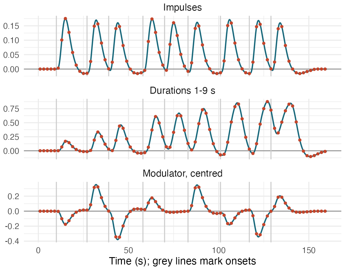
Curves: evaluate() on a 0.1 s grid. Dots: the same regressors at the scan times. Grey vertical lines mark the event onsets.
# Nine events with jittered onsets (s): as brief
# impulses, with durations of 1-9 s, and scaled by a
# mean-centred parametric modulator
ons <- seq(10, 130, by = 15) +
  c(0, 2, -1, 3, 0, -2, 1, 2, -1)
mod <- c(2, 5, 1, 4, 3, 5, 2, 1, 4)
regs <- list(
  "Impulses" = regressor(ons, HRF_SPMG1),
  "Durations 1-9 s" = regressor(ons, HRF_SPMG1,
                                duration = 1:9),
  "Modulator, centred" = regressor(ons, HRF_SPMG1,
                             amplitude = mod - mean(mod))
)

# Scan times for one 80-scan run at TR = 2 s
sf <- sampling_frame(blocklens = 80, TR = 2)
scans <- samples(sf)  # 1, 3, 5, ... (mid-TR)
fine  <- curves(regs, seq(0, 160, by = 0.1))
pts   <- curves(regs, scans)

fig <- ggplot(fine, aes(t, y)) +
  geom_hline(yintercept = 0, colour = "grey60") +
  geom_vline(xintercept = ons, colour = "grey80") +
  geom_line(colour = "#17677a", linewidth = 0.9) +
  geom_point(data = pts, colour = "#c4452b", size = 1.3) +
  facet_wrap(~hrf, ncol = 1, scales = "free_y") +
  labs(x = "Time (s); grey lines mark onsets", y = NULL) +
  theme_show(15) + theme(strip.text = element_text(size = 14))
04
Multi-run designs from run-relative onsets
sampling_frame() records the number of scans in each run and the TR. regressor_design() takes onsets measured from the start of each run, a condition factor and a run index, convolves each run separately, and stacks the runs into one design matrix with a row for every scan.
Here the three runs and 36 events give a 360 × 4 matrix: one row per scan, and two columns, the canonical response and its temporal derivative, for each condition. The columns are named after the condition and basis function. Each run is convolved on its own, so a response stops at the end of its run: the last event of run 1 starts 13 s before the run ends, and the rows of run 2 are the same as when run 2 is built alone.
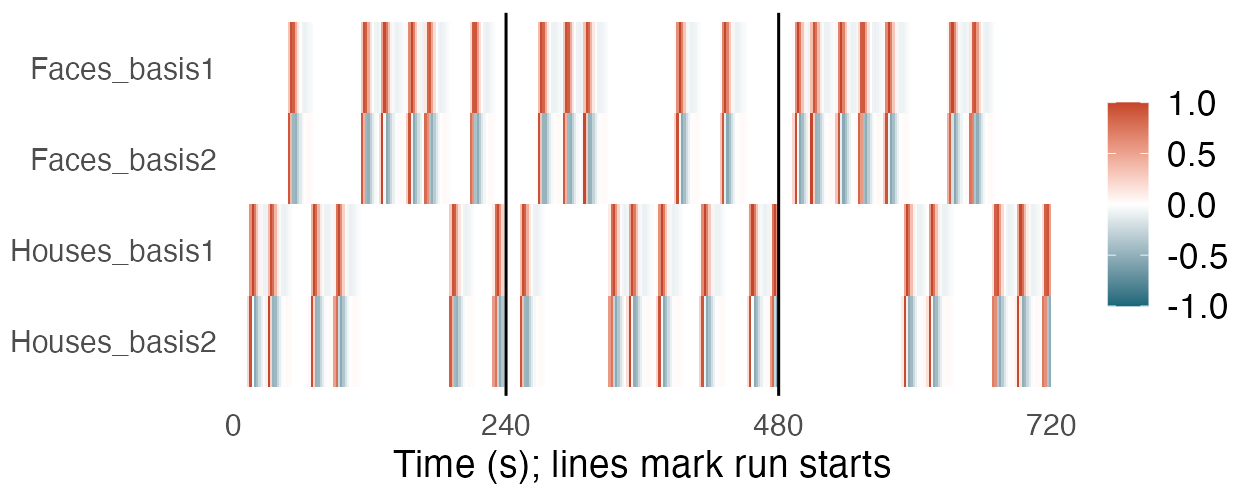
Simulated schedule: 12 events per run, Faces and Houses in random order. Each column is divided by its largest absolute value for display; the derivative columns (_basis2) take negative values.
# Three runs of 120 scans at TR = 2 s. Onsets are given
# relative to the start of their own run.
sf3 <- sampling_frame(blocklens = c(120, 120, 120),
                      TR = 2)
set.seed(7)
ev <- data.frame(
  run   = rep(1:3, each = 12),
  onset = rep(seq(6, 226, by = 20), 3) + runif(36, 0, 6),
  cond  = factor(sample(rep(c("Faces", "Houses"), 18)))
)

# One column per condition and basis function, one row
# per scan; HRF_SPMG2 adds a temporal derivative. Each
# run is convolved separately.
X <- regressor_design(ev$onset, ev$cond, ev$run, sf3,
                      hrf = HRF_SPMG2)
dim(X)       # 360 x 4
colnames(X)  # "Faces_basis1" "Faces_basis2" ...

# Each column scaled to a maximum |value| of 1
Xs <- sweep(X, 2, apply(abs(X), 2, max), "/")
d <- data.frame(t = samples(sf3, global = TRUE),
                col = factor(rep(colnames(X), each = 360),
                             rev(colnames(X))),
                v = as.vector(Xs))
fig <- ggplot(d, aes(t, col, fill = v)) + geom_tile() +
  geom_vline(xintercept = c(240, 480), linewidth = 0.6) +
  scale_fill_gradient2(low = "#17677a", high = "#c4452b",
                       limits = c(-1, 1), name = NULL) +
  scale_x_continuous(breaks = seq(0, 720, 240),
                     expand = c(0, 0)) +
  labs(x = "Time (s); lines mark run starts", y = NULL) +
  theme_show(16) + theme(panel.grid = element_blank(),
                         legend.position = "right")
05
Estimating the response shape with an FIR basis
With hrf = HRF_FIR, regressor_design() returns 12 columns per condition, one for each 2 s bin after an event, and the least-squares coefficients estimate the response in each bin without assuming a shape. The voxel here is simulated on the design from section 04: Faces evoke the canonical HRF delayed by 2 s with lag_hrf(), Houses evoke 60% of that response, and Gaussian noise is added. fmrihrf builds the design but does not fit models; here the fit is base R’s lm() with one baseline per run. fmrireg, which imports fmrihrf, fits fMRI GLMs.
With 18 Faces events across the three runs, the largest FIR coefficient falls in the bin centred at 7 s; the simulated response peaks at 7.0 s. The twelve estimates correlate r = 0.99 with the simulated response averaged over each bin, and 12 of 12 lie within two standard errors of it.
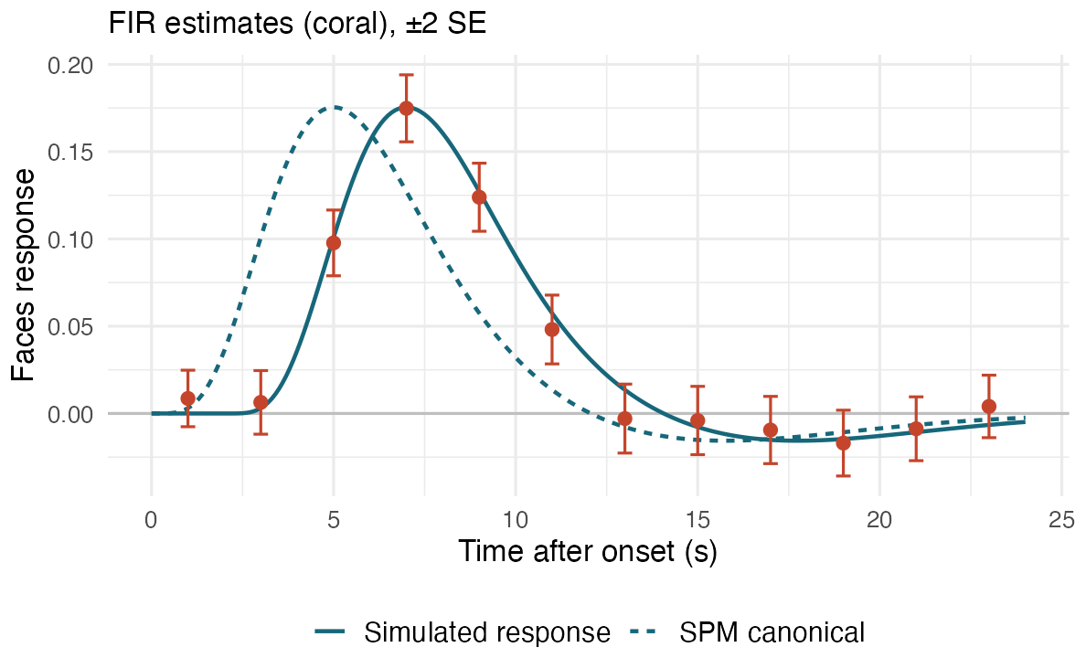
Simulated data. Coral: FIR coefficients for Faces at the bin centres, ±2 standard errors. Solid teal: the simulated response. Dashed teal: the SPM canonical HRF.
# Simulated voxel: Faces evoke a response that peaks
# 2 s later than the canonical HRF; Houses evoke 60% of
# it. Gaussian noise; one baseline per run.
true_hrf <- lag_hrf(HRF_SPMG1, lag = 2)
set.seed(3)
signal <- regressor_design(ev$onset, ev$cond, ev$run,
                           sf3, hrf = true_hrf) %*% c(1, 0.6)
y <- drop(signal) + rnorm(360, sd = 0.03)

# Fit a 12-bin FIR basis: the coefficients estimate the
# response in each 2 s bin after the event
F <- regressor_design(ev$onset, ev$cond, ev$run, sf3,
                      hrf = HRF_FIR)
fit <- lm(y ~ 0 + factor(blockids(sf3)) + F)
# lm() prefixes the matrix name: "FFaces_basis1", ...
faces <- paste0("F", colnames(F)[1:12])
est <- coef(summary(fit))[faces, 1:2]
bins <- data.frame(t = seq(1, 23, by = 2),
                   b = est[, 1], se = est[, 2])

ref <- curves(list("Simulated response" = true_hrf,
                   "SPM canonical" = HRF_SPMG1),
              seq(0, 24, by = 0.1))
fig <- ggplot(bins, aes(t, b)) +
  geom_hline(yintercept = 0, colour = "grey75") +
  geom_line(data = ref, aes(t, y, linetype = hrf),
            colour = "#17677a", linewidth = 0.9) +
  geom_errorbar(aes(ymin = b - 2 * se, ymax = b + 2 * se),
                width = 0.4, colour = "#c4452b") +
  geom_point(colour = "#c4452b", size = 2.4) +
  scale_linetype_manual(values = c("solid", "22"),
                        name = NULL) +
  labs(x = "Time after onset (s)", y = "Faces response",
       title = "FIR estimates (coral), ±2 SE") +
  theme_show(14)
Built on fmrihrf
fmrireg fMRI regression models
Development version
The install command above gives the CRAN release. To install the development version from GitHub:
pak::pak("bbuchsbaum/fmrihrf")Every figure on this page is drawn by software/showcase/fmrihrf/make-figures.R in the site’s source, and the code shown with each figure is the code that drew it. Generic plotting helpers used by that code (curves(), draw(), draw_basis(), draw_fir(), the palette and theme) are defined in software/showcase/fmrihrf/helpers.R, which the script loads first.