fmrireg

GitHub

Flexible regression-based fMRI analysis

Installpak::pak('bbuchsbaum/fmrireg')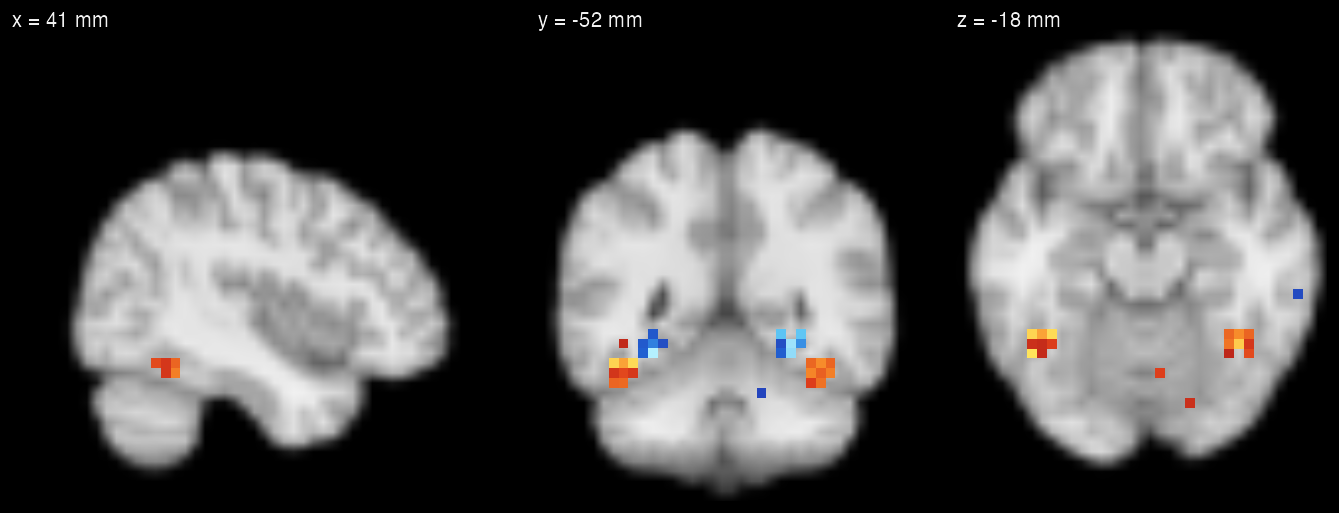

Sagittal, coronal and axial views of the MNI152 template with a face-versus-scene z map thresholded at |z| > 3: simulated bilateral face-region clusters near the fusiform gyrus in red-yellow, parts of the scene-region clusters in blue, and a few isolated false-positive voxels

The face-minus-scene z map from feature 03 below, drawn on neuroim2’s MNI152 template with plot_ortho(style = "dark") in make-figures.R.

Model specification onset ~ hrf(condition) with run blocks and a drift model

Estimation fmri_lm(): OLS, AR prewhitening, robust weighting

Inference Contrasts, t, z and F statistics, maps as NeuroVol

Beyond the canonical GLM HRF estimation, single-trial betas, group meta-analysis

What it does

A formula becomes a design matrix

event_model() turns an event table and a formula such as onset ~ hrf(condition) into one HRF-convolved regressor per condition, sampled at each scan of each run. baseline_model() adds drift terms and a mean for each run; here a cubic B-spline, three columns per run. Both come from the sibling package fmridesign and are re-exported by fmrireg, so the formula you write here is the one fmri_lm() accepts.

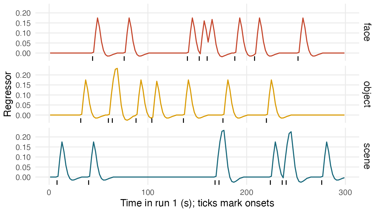
Three convolved regressors for face, object and scene events over the first run, each in its own panel with onset ticks underneath

Simulated design: two runs of 150 scans (TR 2 s), 8 events per condition per run.

library(fmrireg)
library(ggplot2)

# Simulated experiment: two runs of 150 volumes (TR 2 s),
# each with 8 face, 8 scene and 8 object events
set.seed(1)
events <- do.call(rbind, lapply(1:2, function(r) {
  data.frame(run = r,
             onset = sort(sample(seq(8, 280, 4), 24)),
             condition = sample(rep(c("face", "scene",
                                      "object"), 8)))
}))
events$condition <- factor(events$condition)
sframe <- sampling_frame(blocklens = c(150, 150), TR = 2)

# Task regressors from a formula; drift and run means
# from a baseline model (cubic B-spline per run)
emod <- event_model(onset ~ hrf(condition),
                    data = events, block = ~ run,
                    sampling_frame = sframe)
bmod <- baseline_model(basis = "bs", degree = 3,
                       sframe = sframe)
dim(design_matrix(emod))  # 300 x 3
dim(design_matrix(bmod))  # 300 x 8

# The convolved task regressors in run 1
X1 <- as.matrix(design_matrix(emod))[1:150, ]
ts <- data.frame(t = rep(samples(sframe)[1:150], 3),
                 condition = rep(levels(events$condition),
                                 each = 150),
                 y = as.vector(X1))
fig <- ggplot(ts, aes(t, y, colour = condition)) +
  geom_line(linewidth = 0.7) +
  geom_rug(aes(onset), data = subset(events, run == 1),
           inherit.aes = FALSE, length = unit(0.08, "npc")) +
  facet_grid(condition ~ .) + scale_colour_lm() +
  labs(x = "Time in run 1 (s); ticks mark onsets",
       y = "Regressor") + theme_lm()

Simulated data with a known answer

The examples below are fitted to data simulated so that the right answer is known. Two face regions respond most to faces, two scene regions to scenes, and both respond weakly to objects; every voxel has AR(1) noise. The simulated responses peak 1.5 s later than the canonical HRF that the models assume, through hrf(..., lag = 1.5).

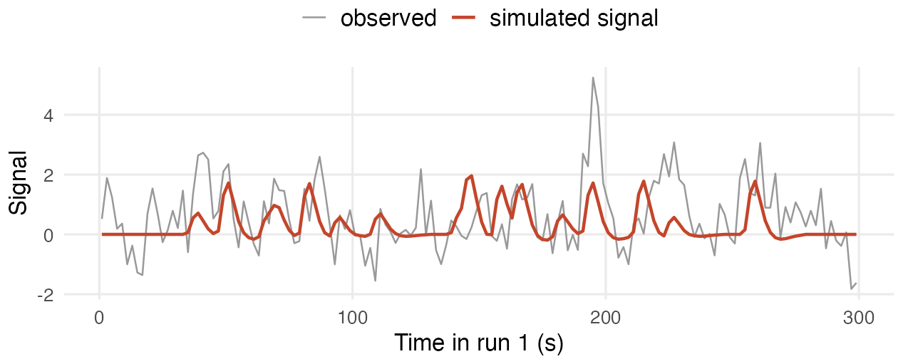
Time series of one face-region voxel over run 1: noisy observed signal in grey with the simulated response, a train of peaks up to about 2, in red

Simulated data: one face-region voxel, run 1.

library(neuroim2)

# Brain mask on neuroim2's MNI152 template (4 mm voxels)
f <- system.file("extdata", "mni_downsampled.nii.gz",
                 package = "neuroim2")
mni <- read_vol(f)
sp  <- space(mni)
mask <- LogicalNeuroVol(
  as.array(mni > quantile(mni[mni > 0], 0.25)), sp)

# Face and scene regions: 8 mm spheres in each hemisphere
sphere <- function(xyz) grid_to_index(sp, coords(
  spherical_roi(mask, coord_to_grid(sp, rbind(xyz)),
                radius = 8)))
vox <- which(as.array(mask))
in_face  <- vox %in% c(sphere(c(40, -52, -18)),
                       sphere(c(-40, -52, -18)))
in_scene <- vox %in% c(sphere(c(28, -44, -8)),
                       sphere(c(-28, -44, -8)))

# Responses peak 1.5 s later than the canonical HRF.
# Signal is scaled so the largest regressor value is
# 2.5 SDs of the AR(1) noise innovations (phi = 0.4).
true_X <- as.matrix(design_matrix(event_model(
  onset ~ hrf(condition, lag = 1.5), data = events,
  block = ~ run, sampling_frame = sframe)))
B <- matrix(0, 3, length(vox))  # face, object, scene
B[, in_face]  <- c(1.0, 0.4, 0.0)
B[, in_scene] <- c(0.0, 0.4, 1.0)
signal <- true_X %*% B * 2.5 / max(true_X)
noise  <- apply(matrix(rnorm(length(signal)), 300), 2,
                stats::filter, filter = 0.4,
                method = "recursive")
Y <- signal + noise

# One face-region voxel in run 1 (plotting helper)
fig <- plot_voxel(Y, signal, which(in_face)[1], 1:150)

Fitting every voxel and mapping a contrast

fmri_lm() fits the model to an fmri_frame; neurovec_frame() builds one from neuroim2 NeuroVec runs and a mask. By default fmri_lm() fits each run separately and combines the runs by fixed-effect meta-analysis, so test statistics are z values. Contrasts declared in the formula, here pair_contrast() for faces minus scenes, are estimated with the coefficients. coef_image() returns the estimate, standard error, test statistic or p of any coefficient or contrast as a NeuroVol on the mask’s grid, ready for neuroim2’s plotting and clustering.

The mask holds 25,277 voxels; the two face regions hold 48 of them and the two scene regions 54. The median z is 4.4 in the face regions and −3.6 in the scene regions. Outside them, where there is no effect, 87 of 25,175 voxels pass |z| > 3, about 68 expected by chance.

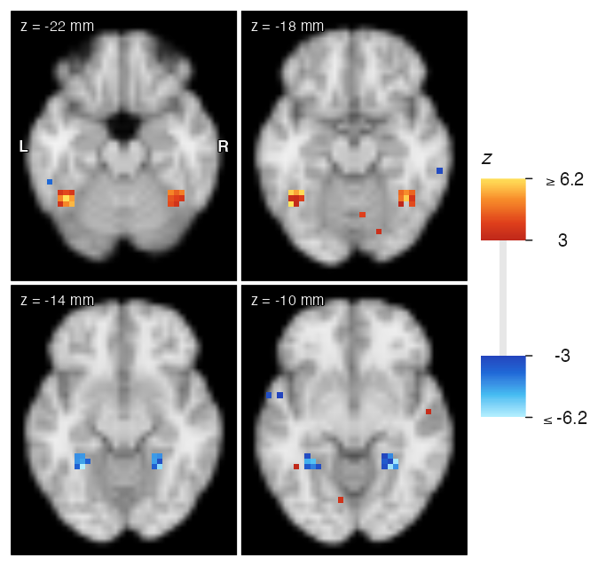
Four axial slices of the template from z = -22 to -10 mm with the face-versus-scene z map thresholded at |z| > 3: positive face-region clusters in red-yellow at z = -22 and -18 mm, negative scene-region clusters in blue at z = -14 and -10 mm

Simulated data: face regions centred at (±40, −52, −18) mm, scene regions at (±28, −44, −8) mm, 8 mm radius. Threshold |z| > 3, uncorrected.

# One NeuroVec per run, then an fmri_frame over the mask
runs <- lapply(1:2, function(r) {
  SparseNeuroVec(Y[(r - 1) * 150 + 1:150, ],
                 add_dim(sp, 150), mask,
                 orientation = "time_x_voxels")
})
dset <- neurovec_frame(runs, mask, TR = 2,
                       event_table = events)

# Fit the GLM with AR(1) prewhitening and one contrast
fvs <- pair_contrast(~ condition == "face",
                     ~ condition == "scene",
                     name = "face_vs_scene")
fit <- fmri_lm(onset ~ hrf(condition, contrasts = fvs),
               block = ~ run, baseline_model = bmod,
               dataset = dset,
               control = fmri_lm_control(
                 noise = noise_spec("ar1")))

# Runs are fitted separately and pooled by fixed-effect
# meta-analysis, so the contrast's statistic is a z value
# ("tstat" is fmri_lm's name for that statistic)
tmap <- coef_image(fit, "face_vs_scene",
                   statistic = "tstat", type = "contrasts")
fig <- plot_overlay(mni, tmap, ov_thresh = 3,
                    ov_symmetric = TRUE, unit = "mm",
                    zlevels = seq(-22, -10, by = 4),
                    ncol = 2, cbar_title = "z")

Prewhitening for autocorrelated noise

noise_spec("ar1") passed through fmri_lm_control() estimates an AR(1) coefficient for each run from residual autocovariances pooled across voxels, whitens the data and the design, and refits. noise_spec("iid") gives ordinary least squares. With positively autocorrelated noise, OLS standard errors are too small and null p-values pile up near zero.

Both runs’ AR(1) estimates are 0.400 (simulated 0.4); pooling over 25,277 voxels makes them precise. Among the 25,175 voxels with no effect, 15.1% reach p < 0.05 under OLS and 5.2% after prewhitening (two-sided tests of the z statistic that combines the two runs).

Two histograms of p-values for the face-versus-scene contrast in voxels with no effect: under OLS the counts are highest near zero and fall off; after AR(1) prewhitening they are flat at the dashed line expected for uniform p-values

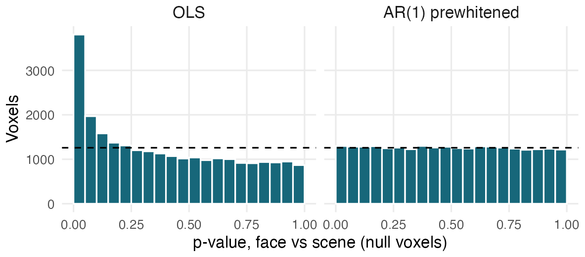
Simulated data. Dashed line: the count per bin if p-values were uniform.

# The same model without prewhitening (OLS)
fit_ols <- fmri_lm(onset ~ hrf(condition, contrasts = fvs),
                   block = ~ run, baseline_model = bmod,
                   dataset = dset,
                   control = fmri_lm_control(
                     noise = noise_spec("iid")))

fit$ar_coef  # one AR(1) coefficient per run

# Voxels outside both regions have no face-scene
# difference, so their p-values should be uniform
null <- !in_face & !in_scene
p_of <- function(m) p_values(m, type = "contrasts")[[1]]
pv <- data.frame(
  p = c(p_of(fit_ols)[null], p_of(fit)[null]),
  model = rep(c("OLS", "AR(1) prewhitened"),
              each = sum(null)))
pv$model <- factor(pv$model, unique(pv$model))

fig <- ggplot(pv, aes(p)) +
  geom_histogram(breaks = seq(0, 1, 0.05),
                 fill = "#17677a", colour = "white") +
  geom_hline(yintercept = sum(null) / 20,
             linetype = "dashed") +
  facet_wrap(~ model) +
  labs(x = "p-value, face vs scene (null voxels)",
       y = "Voxels") +
  theme_lm()

Estimating the response shape

estimate_hrf() estimates one response curve per condition with a penalised cubic B-spline basis (eight functions per curve by default), choosing one smoothing parameter for all voxels by generalised cross-validation. Curves are constrained to zero at the first and last time in rsam. The result is a check on the canonical HRF assumed in the fits above.

The estimated face response peaks at 7.0 s after onset, against 6.5 s in the simulation and 5.0 s for the canonical HRF; its peak height is 1.80, against 1.82 simulated.

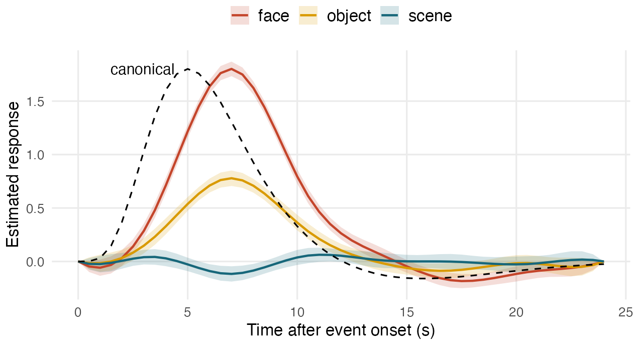
Estimated response curves for face, object and scene events in the face regions: face peaks near 7 s at about 1.8, object near 7 s at about 0.8, scene stays within about 0.1 of zero; a dashed canonical HRF scaled to the face peak rises and peaks about 2 s earlier

Simulated data: mean signal of the face regions. Bands are 95% intervals that assume independent errors, so they are too narrow for this AR(1) noise.

# Estimate the response shape in the face regions with
# a smooth spline basis, without assuming its form
roi <- matrix_frame(matrix(rowMeans(Y[, in_face])),
                    TR = 2, run_length = c(150, 150),
                    event_table = events)
est <- estimate_hrf(onset ~ hrf(condition),
                    block = ~ run, dataset = roi,
                    basemod = bmod, rsam = seq(0, 24, 0.5))
curves <- tidy(est)
curves$condition <- sub("condition.", "", curves$curve)

# Canonical HRF (dashed), scaled to the face peak
canon <- fmrihrf::HRF_SPMG1(est$time)
peak  <- max(curves$estimate)
canon <- data.frame(time = est$time,
                    y = canon / max(canon) * peak)

fig <- ggplot(curves, aes(time, estimate)) +
  geom_ribbon(aes(ymin = lower, ymax = upper,
                  fill = condition), alpha = 0.18) +
  geom_line(aes(colour = condition), linewidth = 0.9) +
  geom_line(aes(y = y), data = canon, linetype = "dashed") +
  annotate("text", x = 4.4, y = peak, hjust = 1,
           label = "canonical", size = 4.5) +
  scale_colour_lm() + scale_fill_lm() +
  labs(x = "Time after event onset (s)",
       y = "Estimated response", colour = NULL,
       fill = NULL) +
  theme_lm(legend = "top")

Built on

neuroim2 Volumes, masks and images of results

fmrihrf Hemodynamic response functions

fmridesign Event and baseline models, contrasts

fmridataset The fmri_frame data container

fmriAR AR and ARMA noise estimation and whitening

fmrilss Least-squares-separate single-trial estimation

Every figure on this page, including the hero, is drawn by software/showcase/fmrireg/make-figures.R in the site’s source, and the code shown with each figure is the code that drew it. Colours, theme and the single-voxel plot in feature 02 come from styling helpers in software/showcase/fmrireg/helpers.R.