neurocluster

GitHub

Spatially constrained clustering for neuroimaging

Installpak::pak('bbuchsbaum/neurocluster')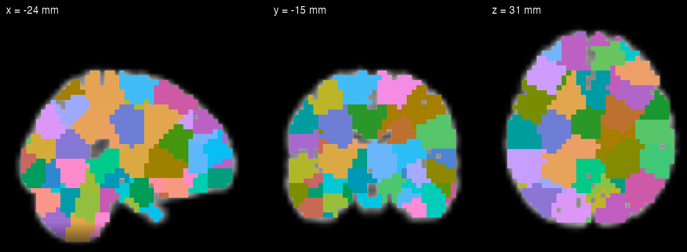

Sagittal, coronal and axial views of the MNI152 template covered by about two hundred compact parcels, each in its own colour

A 200-parcel SLIC fit to a simulated run on neuroim2’s MNI152 template, drawn with neuroim2’s plot_ortho(style = "dark"). The same fit appears in sections 03 and 04.

Entry point cluster4d(): 4D data and a mask in, labelled parcels out

Methods 13, including ReNA, ACSC, SLIC, SNIC, G3S and FLASH-3D

Checks validate_cluster4d(), cluster_metrics(), compare_cluster4d()

Output Label volume, parcel mean time series, centroids in mm

What it does

One call fits a parcellation

cluster4d() takes a NeuroVec and a mask and returns a cluster4d_result: one label per mask voxel, the labels as a ClusteredNeuroVol, the mean time series of each parcel (centers) and each parcel’s centroid in millimetres (coord_centers). The method argument selects one of 13 algorithms; n_clusters is a target, and actual_k records how many parcels the method returned. validate_cluster4d() recomputes the centres and geometry from the original inputs and checks them against the result.

The simulated run has 25,277 brain voxels and 60 volumes on the template’s 4 mm grid. ReNA, asked for 12 parcels, returned 12; validate_cluster4d() reports the result as valid, and the adjusted Rand index against the simulated regions is 0.993.

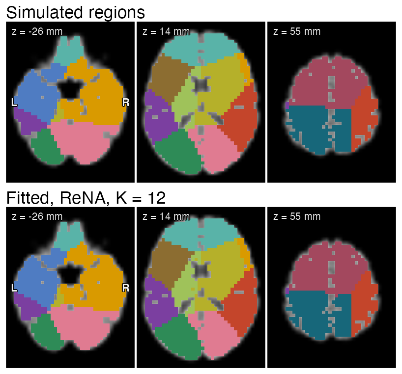
Two rows of three axial slices. The top row shows twelve simulated regions in distinct colours; the bottom row shows the fitted parcels, which match the simulated regions almost voxel for voxel

Simulated data: 12 regions, each with its own unit-variance random signal, plus independent voxel noise with SD 1.5. Fitted IDs are matched to simulated ones by maximum overlap for display only.

library(neuroim2)
library(neurocluster)

# neuroim2's MNI152 template, downsampled to ~4 mm voxels
f <- system.file("extdata", "mni_downsampled.nii.gz",
                 package = "neuroim2")
mni  <- read_vol(f)
mask <- (mni > quantile(mni[mni > 0], 0.25)) * 1

# 12 regions: each voxel joins the nearest of 12 seeds
set.seed(1)
idx   <- which(as.array(mask) > 0)
xyz   <- index_to_coord(mask, idx)            # mm
truth <- FNN::get.knnx(xyz[sample(nrow(xyz), 12), ],
                       xyz, k = 1)$nn.index[, 1]

# One unit-variance signal per region; runs differ
# only in the voxel noise (SD 1.5) drawn for them
n_t <- 60
sig <- matrix(rnorm(12 * n_t), 12, n_t)
simulate <- function(seed, noise_sd = 1.5) {
  set.seed(seed)
  X <- sig[truth, ] + rnorm(length(idx) * n_t, sd = noise_sd)
  run <- matrix(0, prod(dim(mni)), n_t)
  run[idx, ] <- X
  list(X = X, vec = NeuroVec(array(run, c(dim(mni), n_t)),
                             add_dim(space(mni), n_t)))
}
sim <- simulate(1)
fit <- cluster4d(sim$vec, mask, n_clusters = 12,
                 method = "rena", connectivity = 26)
validate_cluster4d(fit, sim$vec, mask)$valid
cluster_metrics(fit, truth = truth)$ari_truth
fig <- show_pair(truth, fit$labels)

Methods compared on identical voxels

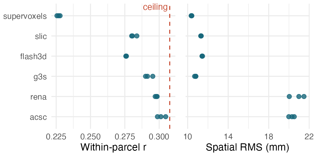
compare_cluster4d() first checks that every result covers the same mask voxels in the same physical space, then returns a data frame of the estimands requested: parcel counts and sizes, spatial RMS distance from each voxel to its parcel centroid in millimetres, and the mean Pearson correlation over all within-parcel voxel pairs (which needs the voxel time series). Here six methods are fitted to the simulated run from section 01 and two more like it, with 200 parcels each and every other setting at its default.

Each method is fitted to three simulated runs that share regions and signals and differ only in their noise; the table gives the range over the three runs, and every fit returned 200 parcels. The dashed line is the ceiling 1 / (1 + 1.5²) = 0.308: the expected correlation between two voxels of the same region, and so the most a parcel that never crosses a region border can reach on average.

This shows how to compare methods on your own data, not which method to choose: results depend on K, on the data, and on spatial_weight, which maps to a different parameter in each method.

Two dot plots with one row per method, in the order supervoxels, slic, flash3d, g3s, rena, acsc, and one point per simulated run: mean within-parcel correlation with a dashed ceiling line, and spatial RMS distance in millimetres

Method	Within-parcel r	RMS (mm)
`supervoxels`	0.226–0.228	10.3–10.4
`slic`	0.280–0.284	11.3
`flash3d`	0.276	11.4–11.5
`g3s`	0.290–0.295	10.7–10.8
`rena`	0.297–0.299	20.0–21.5
`acsc`	0.299–0.305	20.0–20.5

Simulated data, default settings. Methods are listed in the order of ?cluster4d; ranges are over three runs.

# Six methods, 200 parcels each, on three simulated
# runs; every other setting is left at its default
methods <- c("supervoxels", "slic", "flash3d", "g3s",
             "rena", "acsc")
cmp <- do.call(rbind, lapply(1:3, function(seed) {
  run  <- simulate(seed)
  fits <- lapply(methods, function(m)
    cluster4d(run$vec, mask, n_clusters = 200,
              method = m))
  # Checks that all fits share voxels and geometry
  out <- compare_cluster4d(fits,
    metrics = c("summary", "spatial_dispersion",
                "temporal_coherence"),
    feature_mat = run$X)
  cbind(out, method = methods, run = seed)
}))

# Expected r between two voxels of one region: the
# ceiling for mean within-parcel correlation
ceiling <- 1 / (1 + 1.5^2)
fig <- method_panels(cmp, methods, ceiling)

Above 0.3, `spatial_weight` trades boundary fidelity for compactness

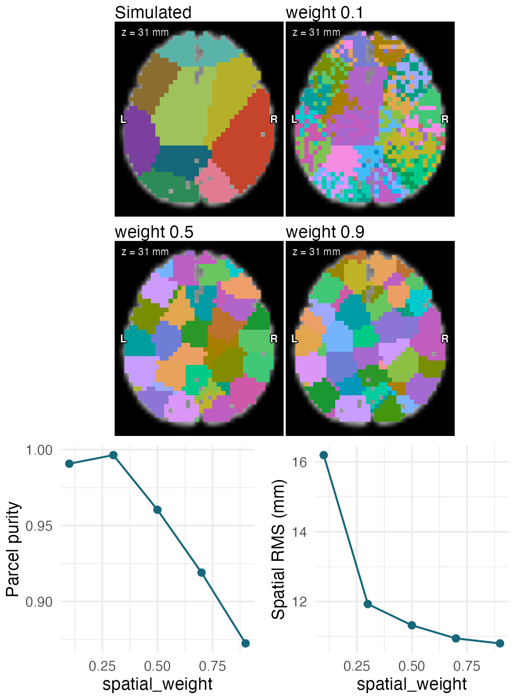
spatial_weight (0 to 1, default 0.5) sets how much spatial distance counts against signal similarity. Most methods map it to a parameter of their own (ReNA and ReNA++ do not use it); for SLIC it sets compactness = 20 * spatial_weight. The sweep fits 200 parcels, finer than the 12 simulated regions, at five weights. Parcel purity is the share of voxels whose parcel’s majority region is their own region.

Asked for 200 parcels, SLIC returned 211 at weight 0.1 and 200 at the other weights; n_clusters is a target, and refitting with preserve_k = TRUE returns 200 at 0.1. In every fit each parcel is a single 26-connected piece of the mask. Purity peaks at weight 0.3 (99.6%), with voxels 11.9 mm (RMS) from their parcel centroid. Above 0.3, each increase makes parcels more compact and less pure, reaching 10.8 mm and 87.2% at 0.9. At 0.1, purity is 99.1%, but the parcels are irregular, with an RMS distance of 16.2 mm.

Top: one axial slice showing the simulated regions and SLIC parcels at spatial weights 0.1, 0.5 and 0.9; parcels are irregular and interleaved at 0.1 and compact at 0.9. Bottom: parcel purity is near 0.99 at weights 0.1 and 0.3 and falls to about 0.87 at 0.9, while spatial RMS distance falls from about 16 mm to 11 mm

# 200 parcels, finer than the 12 simulated regions.
# spatial_weight trades signal similarity against
# distance; for SLIC, compactness = 20 * spatial_weight
weights <- c(0.1, 0.3, 0.5, 0.7, 0.9)
sweep <- lapply(weights, function(w)
  cluster4d(sim$vec, mask, n_clusters = 200,
            method = "slic", spatial_weight = w))

# Share of voxels whose parcel's majority region is
# their own region: 1 when no parcel crosses a border
purity <- function(lab) {
  tab <- table(lab, truth)
  sum(apply(tab, 1, max)) / length(lab)
}
res <- data.frame(
  weight = weights,
  k      = sapply(sweep, `[[`, "actual_k"),
  purity = sapply(sweep, function(f) purity(f$labels)),
  rms    = sapply(sweep, function(f)
    cluster_metrics(f)$spatial_rms_distance_mm))

fig <- sweep_figure(res, sweep, weights)

Parcel time series and a NIfTI label map

The result’s clusvol is a neuroim2 ClusteredNeuroVol, so write_vol() saves the parcellation as NIfTI, and centers holds one mean time series per parcel for connectivity or other parcel-level analyses.

fit200$centers is a 200 × 60 matrix (parcels × volumes) in the original signal units. Parcels assigned to the same simulated region correlate at a mean r = 0.96, parcels in different regions at r = 0.01. The NIfTI file read back with read_vol() reproduces the labels exactly.

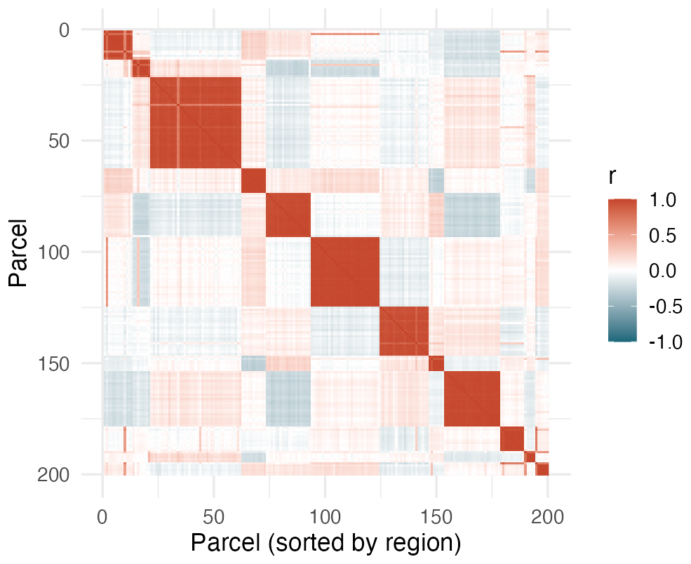
A 200 by 200 correlation matrix of parcel mean time series, sorted by simulated region, with high-correlation red blocks along the diagonal, one per region

Correlations between the parcel means of the spatial_weight 0.5 fit. Each red block on the diagonal is the set of parcels lying mostly within one simulated region.

# The weight 0.5 fit: labels as a NIfTI volume, and
# one mean time series per parcel
fit200 <- sweep[[3]]
out <- tempfile(fileext = ".nii.gz")
write_vol(fit200$clusvol, out)
dim(fit200$centers)      # parcels x volumes

# Parcel-by-parcel correlation, parcels sorted by the
# simulated region that holds most of their voxels
region <- apply(table(fit200$labels, truth), 1,
                which.max)
ord <- order(region)
r   <- cor(t(fit200$centers))[ord, ord]
library(ggplot2)
df  <- data.frame(i = c(row(r)), j = c(col(r)),
                  r = c(r))
fig <- ggplot(df, aes(i, j, fill = r)) +
  geom_raster() +
  scale_fill_gradient2(low = "#17677a", mid = "white",
                       high = "#c4452b",
                       limits = c(-1, 1)) +
  scale_y_reverse() + coord_fixed() +
  labs(x = "Parcel (sorted by region)", y = "Parcel",
       fill = "r") +
  theme_minimal(base_size = 15)

Built on

neuroim2 Image classes, NIfTI input and output

Every figure on this page is drawn by software/showcase/neurocluster/make-figures.R in the site’s source, and the code shown with each figure is the code that fitted and measured it; plotting helpers are in plot-helpers.R in the same folder.