neuroim2

CRAN

Core neuroimaging data structures for fMRI analysis in R

Installinstall.packages('neuroim2')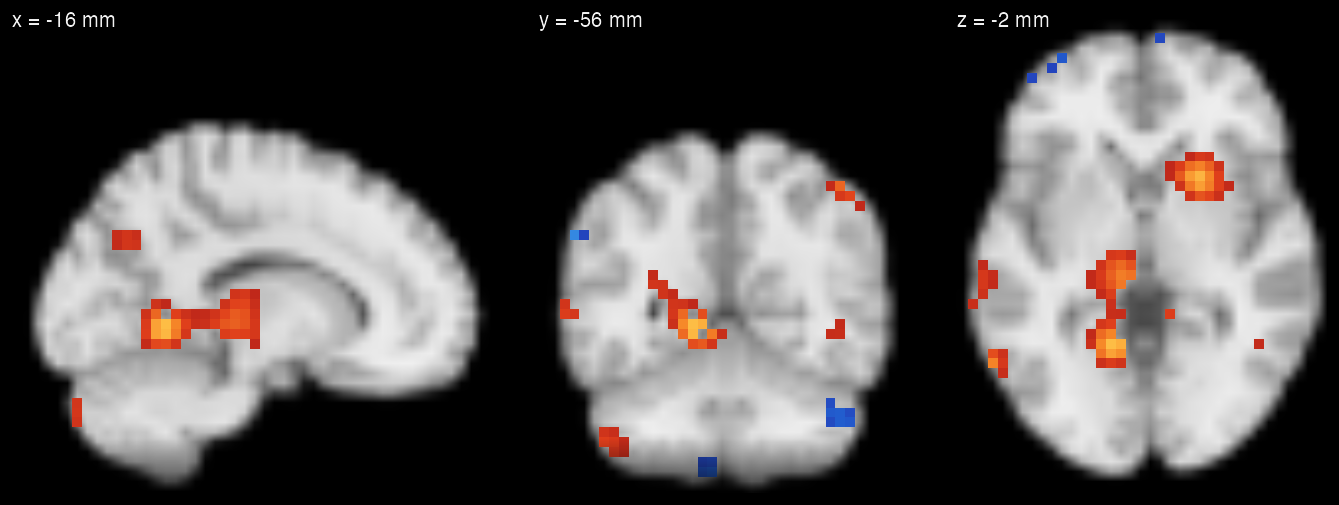

Sagittal, coronal and axial views of the MNI152 template with a thresholded simulated statistic map: positive values in red-yellow, negative in blue

A simulated statistic map on the package’s MNI152 template, drawn with plot_ortho(style = "dark"). Every figure on this page is real package output.

Classes NeuroVol · NeuroVec · NeuroSpace · ROI

Input / output NIfTI read and write, memory-mapped 4D data

Spatial operations Smoothing, resampling, connected components

Analysis building blocks Spherical ROIs, searchlight iterators, ROI time series

What it does

Images that know where they are

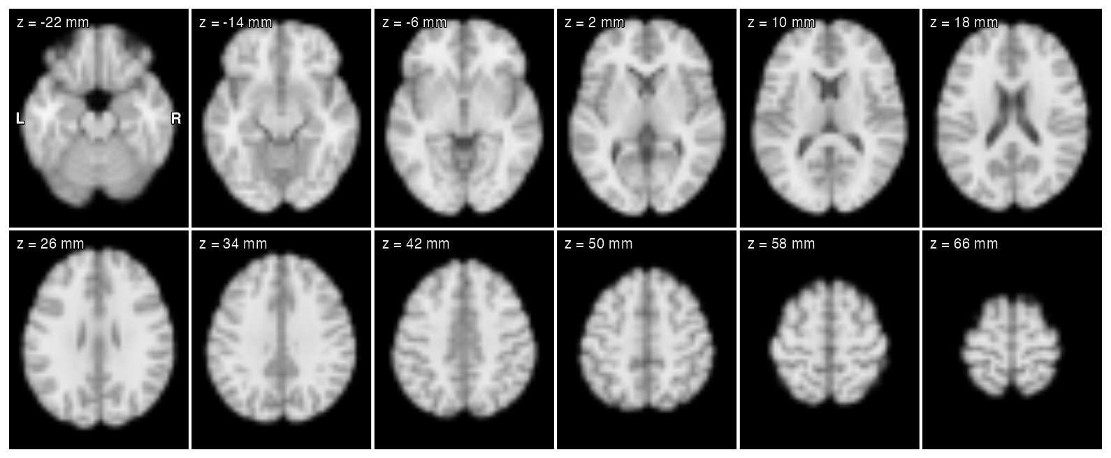
A NeuroVol carries its grid, voxel spacing, origin and orientation with the data, so slicing, plotting and resampling stay in world coordinates.

Twelve axial slices of the MNI152 template arranged in two rows

library(neuroim2)

# A downsampled MNI152 template ships with the package.
# It is a 4 mm grid whose header records 1 mm voxels,
# so we restate the spacing explicitly.
f <- system.file("extdata", "mni_downsampled.nii.gz",
                 package = "neuroim2")
mni <- read_vol(f)
sp  <- NeuroSpace(dim(mni), spacing = c(4, 4, 4),
                  origin = origin(space(mni)))
mni <- NeuroVol(as.array(mni), sp)
space(mni)  # grid, spacing, origin, orientation

fig <- plot_montage(mni, n_slices = 12, ncol = 6)

Smoothing in millimetres

Kernels are specified in physical units (here, FWHM in mm), and statistic maps overlay directly on anatomy with a symmetric diverging scale.

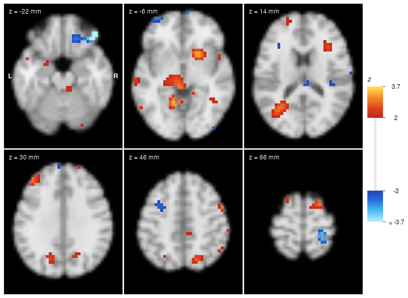
Six axial slices of the template with a thresholded simulated z map: positive values in red-yellow, negative in blue

Simulated data: smoothed Gaussian noise, thresholded at |z| > 2.

# Simulated statistic map: Gaussian noise inside the
# brain, smoothed to 16 mm FWHM
set.seed(2)
mask  <- mni > quantile(mni[mni > 0], 0.25)
noise <- NeuroVol(rnorm(prod(dim(mni))), space(mni))
stat  <- gaussian_blur(noise, mask, fwhm = 16)
stat  <- stat / sd(stat[mask > 0])  # unit variance

fig <- plot_overlay(mni, stat, ov_thresh = 2,
                    ov_symmetric = TRUE, n_slices = 6,
                    ncol = 3, cbar_title = "z")

Clusters, with the table to match

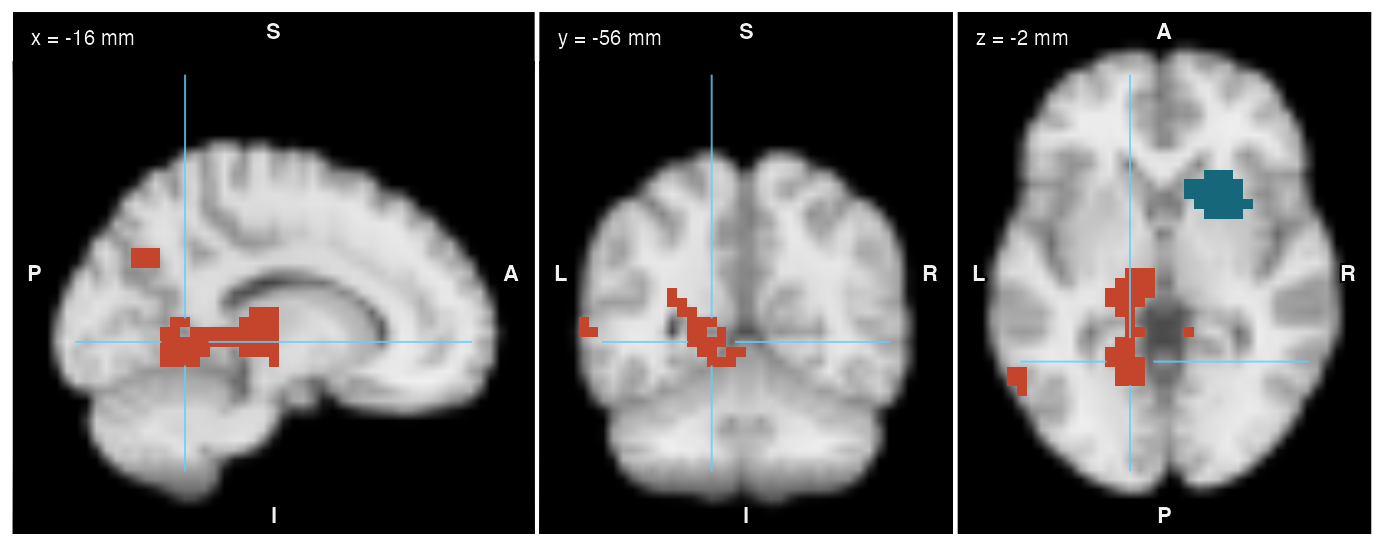
conn_comp() labels connected components above a threshold and returns a cluster table: size, volume and peak location for each component.

Orthogonal views through the peak of the largest cluster; cluster 1 in coral and cluster 2 in teal, matching the table

Cluster	Voxels	Volume (mm³)	Peak (x, y, z mm)	Peak z
1	307	19,648	(-16, -56, -2)	3.45
2	126	8,064	(20, 12, -2)	3.38
3	63	4,032	(-48, 36, 26)	3.08
4	62	3,968	(20, -76, 58)	3.04
5	32	2,048	(20, 4, 66)	2.89

The five largest clusters where z > 2 in the simulated map; colours match the figure. Clusters 3–5 lie outside these three slices. Volumes use the template’s 4 mm voxels.

# Connected components where z > 2, with a cluster table
cc   <- conn_comp(stat, threshold = 2, cluster_table = TRUE)
top5 <- head(cc$cluster_table, 5)

# Label the five largest clusters 1-5 (NA is transparent)
labels <- NeuroVol(array(NA_real_, dim(mni)), space(mni))
idx <- as.array(cc$index)
for (k in 1:5) labels[idx == top5$index[k]] <- k

# One colour per label: a stepped palette over 0.5-5.5
cols <- c("#c4452b", "#17677a", "#d99a00",
          "#7b3fa0", "#2e8b57")
pal  <- rep(cols, each = 52)[1:256]

peak <- unlist(top5[1, c("x", "y", "z")])  # voxel indices
fig  <- plot_ortho(mni, coord = peak, overlay = labels,
                   ov_cmap = pal, ov_range = c(0.5, 5.5),
                   colorbar = FALSE)

ROIs and searchlights

Spherical and cuboid ROIs are objects with coordinates and values.

searchlight() returns a lazy iterator with one sphere per voxel in the mask (25,277 here), the core of searchlight decoding in rMVPA.

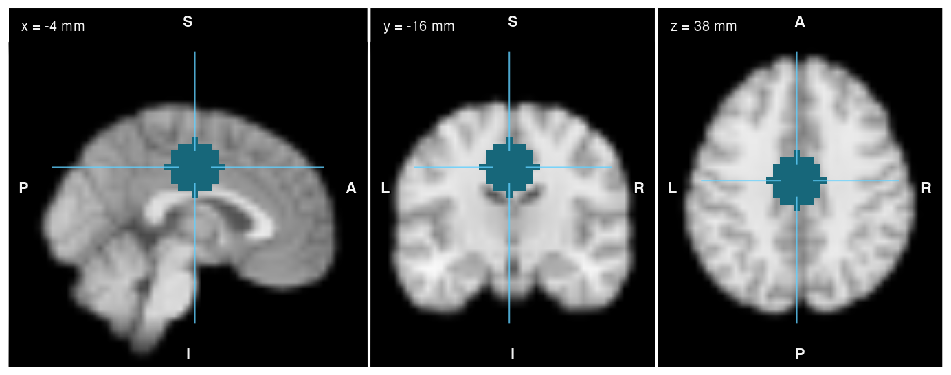
Orthogonal views of the template with a spherical ROI of 16 mm radius highlighted in teal

# Spherical ROIs and searchlights are first-class objects
centre <- c(24, 30, 30)                  # voxel indices
roi <- spherical_roi(mask, centroid = centre,
                     radius = 16, fill = 1)  # radius, mm
sl  <- searchlight(mask, radius = 8)   # lazy iterator

sphere <- NeuroVol(array(0, dim(mni)), space(mni))
sphere[coords(roi)] <- 1
fig <- plot_ortho(mni, coord = centre, overlay = sphere,
                  ov_thresh = 0.5, colorbar = FALSE,
                  ov_cmap = c("#17677a", "#17677a"))

4D runs without loading them

Write a run to NIfTI, map it back from disk, and pull time series for any set of voxels.

The run is 120 volumes on the template grid. Held in memory it is a 120.2 MB R object; memory-mapped, the R object is 0.01 MB and the 60 MB file stays on disk until voxels are read. The mean time course of the 257-voxel ROI tracks the simulated design (r = 0.98).

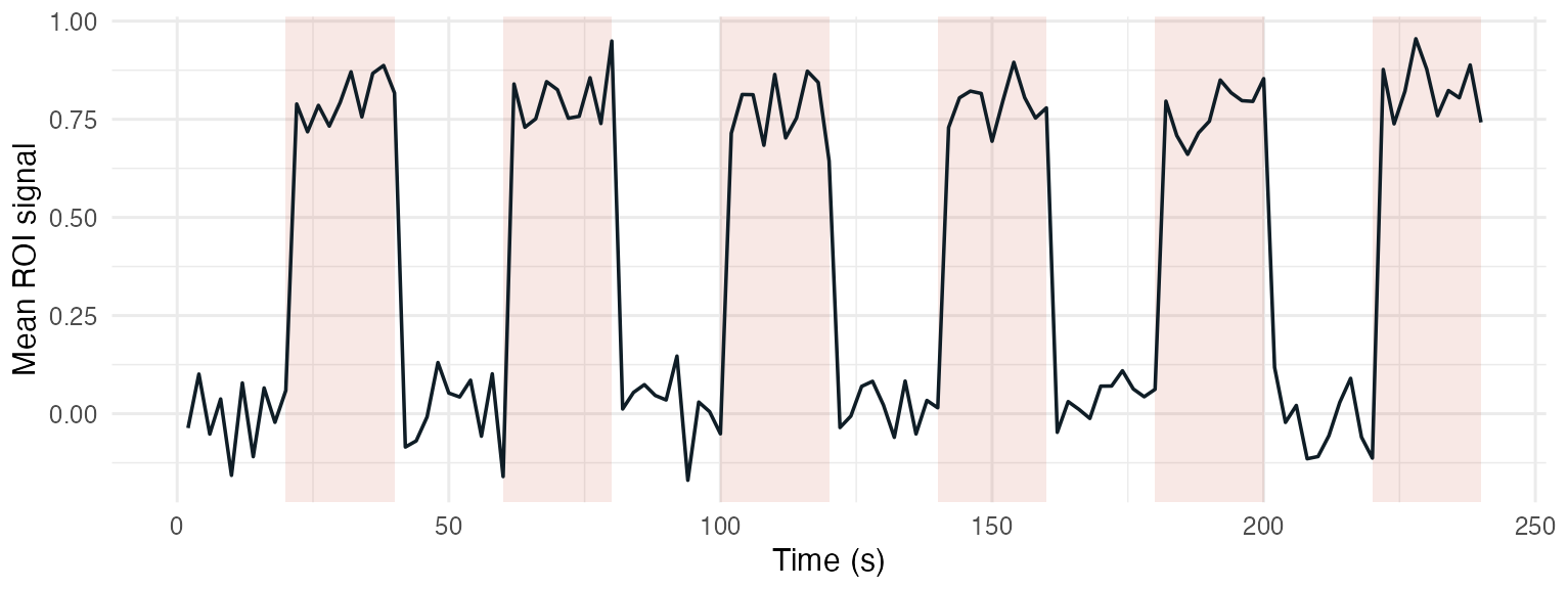
Mean ROI signal over 240 seconds rising during each shaded 20-second block and returning to baseline between blocks

Simulated 4D run: 120 volumes (TR 2 s) with a block design added inside the ROI.

# Simulated 4D run: 120 volumes (TR = 2 s), with a
# 20 s on / 20 s off block design inside the ROI
n_t    <- 120
design <- rep(rep(c(0, 1), each = 10), length.out = n_t)
run    <- array(rnorm(prod(dim(mni)) * n_t),
                c(dim(mni), n_t))
in_roi <- rep(as.array(sphere) > 0, n_t)
run[in_roi] <- run[in_roi] +
  0.8 * rep(design, each = sum(as.array(sphere) > 0))
vec <- NeuroVec(run, add_dim(space(mni), n_t))

# Write to NIfTI, then memory-map it back:
# voxels are read from disk on demand
f <- tempfile(fileext = ".nii")
write_vec(vec, f, data_type = "FLOAT")
mapped <- read_vec(f, mode = "mmap")

roi_ts  <- series(mapped, coords(roi))  # time x voxel
mean_ts <- rowMeans(roi_ts)

library(ggplot2)
df  <- data.frame(t = seq_len(n_t) * 2, y = mean_ts,
                  on = design)
fig <- ggplot(df) +
  geom_rect(aes(xmin = t - 2, xmax = t, ymin = -Inf,
                ymax = Inf, alpha = on * 0.12),
            fill = "#c4452b") +
  scale_alpha_identity() +
  geom_line(aes(t, y), linewidth = 0.7, colour = "#0f1d26") +
  labs(x = "Time (s)", y = "Mean ROI signal") +
  theme_minimal(base_size = 13)

Built on neuroim2

fmrireg fMRI regression models

rMVPA Multivariate pattern analysis

neurosurf Cortical surface data

neuroatlas Atlases and parcellations

Development version

The CRAN release is shown above. To install the development version from GitHub:

pak::pak("bbuchsbaum/neuroim2")

Every figure on this page is drawn by software/showcase/neuroim2/make-figures.R in the site’s source, and the code shown is the code that produced each figure.