rMVPA

GitHub

Multivariate pattern analysis of fMRI data

Installpak::pak('bbuchsbaum/rMVPA')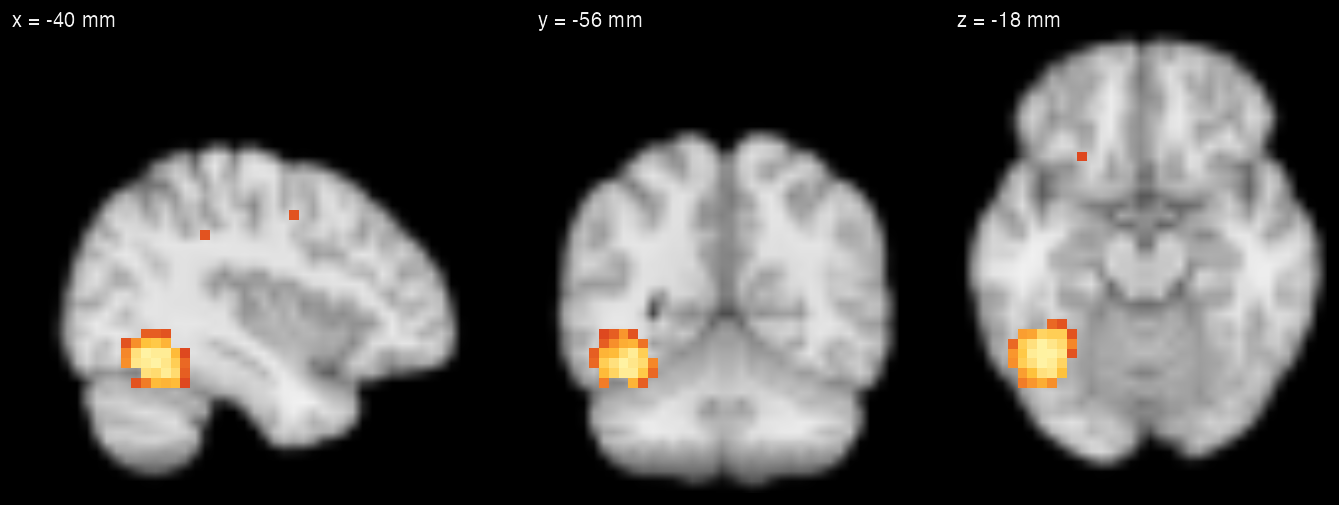

Sagittal, coronal and axial views of the MNI152 template with a searchlight accuracy map in red-yellow: a compact region of high accuracy in left ventral occipitotemporal cortex and a few isolated voxels elsewhere

A searchlight decoding map from run_searchlight() on simulated data, drawn with neuroim2’s plot_ortho(style = "dark") in make-figures.R. Voxels with accuracy of at least 0.5 are shown; chance is 0.25.

Analyses run_regional() · run_searchlight() · run_global()

Cross-validation Leave-one-run-out, k-fold, bootstrap and custom folds

Methods Classification, regression, RSA with cross-validated distances

Inference Permutation null maps with FDR correction

What it does

An analysis in rMVPA is built from three objects: an mvpa_dataset holds the images and mask, an mvpa_design holds the labels and the run of each observation, and a model specification such as mvpa_model() or rsa_model() holds the estimator and, for mvpa_model(), the cross-validation scheme. The same specification can be run in each region of an atlas with run_regional(), in a sphere around every voxel with run_searchlight(), or on all voxels at once with run_global().

Decoding within a region, one run held out at a time

run_regional() fits the model in each labelled region of a mask and returns a performance_table (accuracy and AUC per region) and a prediction_table with one held-out prediction per observation. blocked_cross_validation() makes each run a test fold, so no test pattern shares a run with the training data. The example uses the Haxby et al. (2001) patterns that ship with the package.

Across the 12 held-out runs the classifier labels 88 of 96 patterns correctly (accuracy 91.7%; chance is 12.5% for eight balanced classes). Per-category accuracy ranges from 75.0% (bottle) to 100.0%.

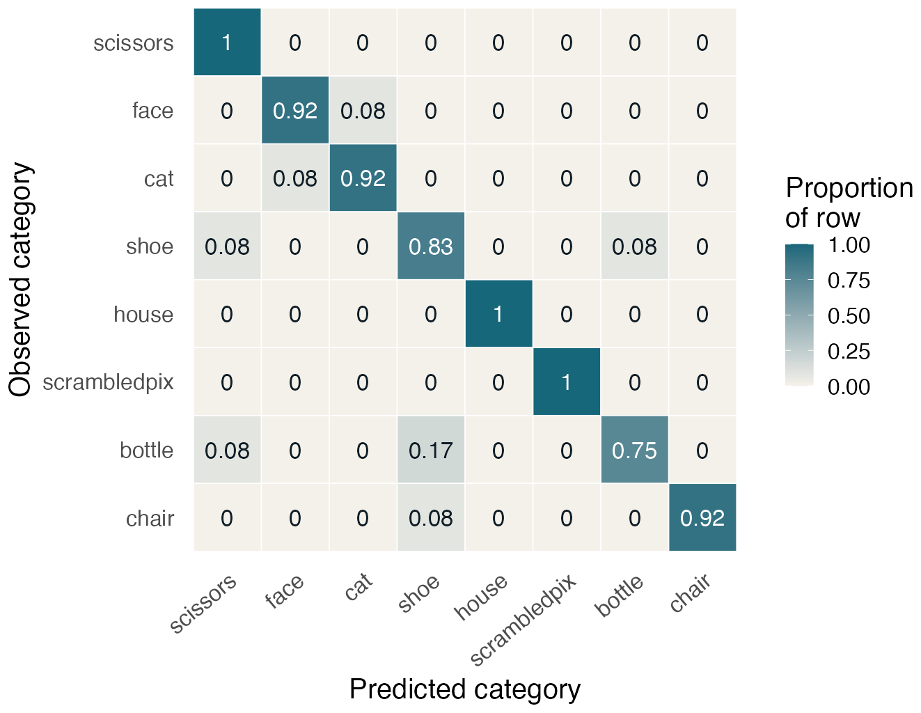
Eight-by-eight confusion matrix of observed against predicted category, with proportions between 0.75 and 1 on the diagonal and small off-diagonal errors, the largest being bottle predicted as shoe at 0.17

Haxby et al. (2001), subject 1: 96 block-mean patterns (one block per category per run) from ventral temporal cortex, classified with shrinkage discriminant analysis (sda_notune). Each row sums to 1.

library(rMVPA)
library(neuroim2)

# Haxby et al. (2001), subject 1, ships with rMVPA: 96
# block-mean patterns (one block per category per run;
# 8 categories x 12 runs) over 577 ventral temporal voxels
hx <- readRDS(system.file("extdata", "haxby2001_subj1",
                          "patterns.rds", package = "rMVPA"))

# Put the voxel columns back into the scanner grid
vt <- array(0L, hx$mask_dim)
vt[hx$mask_idx] <- 1L
vt  <- LogicalNeuroVol(vt, hx$mask_space)
vec <- SparseNeuroVec(t(hx$patterns), mask = vt,
                      space = add_dim(hx$mask_space, 96))

dset <- mvpa_dataset(vec, mask = vt)
des  <- mvpa_design(
  data.frame(category = hx$category, run = hx$run),
  y_train = ~ category, block_var = ~ run)

# Leave one run out: each run is predicted by a model
# fitted to the other 11
mod <- mvpa_model(load_model("sda_notune"), dset, des,
                  crossval = blocked_cross_validation(hx$run))
res <- run_regional(mod, region_mask = vt)
res$performance_table  # Accuracy, AUC

pred <- res$prediction_table  # one row per held-out pattern
fig  <- confusion_plot(pred$observed, pred$predicted)

Searchlight maps from the same model specification

run_searchlight() repeats the cross-validated fit in a sphere around every voxel in the mask (radius in millimetres) and returns one NeuroVol per performance metric. The data here are simulated: unit-variance noise in every voxel, plus a condition-specific pattern inside two 12 mm spheres, one in left ventral occipitotemporal cortex and one in right lateral occipital cortex.

The map has one value for each of the 25,277 voxels in the brain mask. For sda_notune, run_searchlight() selected its sda_fast engine: it computes per-voxel statistics once per fold and reuses them in every sphere, giving the same fits as fitting each sphere separately. The whole map took 17 s on the machine that built this page. The figure shows centres with accuracy of at least 0.5 (chance is 0.25); the highest is 0.98.

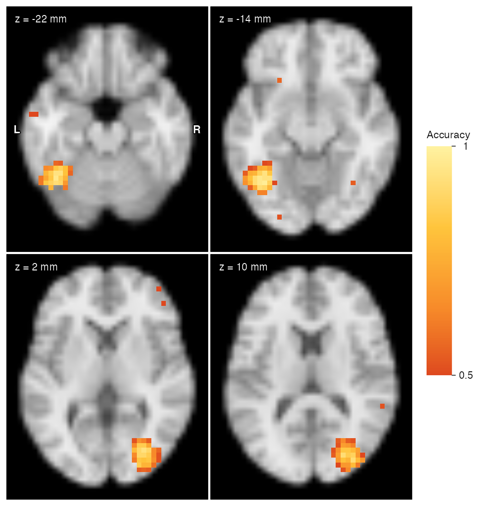
Four axial slices of the template with the searchlight accuracy map: two compact regions of accuracy near 1, in left ventral occipitotemporal and right lateral occipital cortex, and scattered single voxels just above 0.5

Simulated data: four conditions, six runs of eight trials. The isolated voxels above 0.5 outside the two spheres are noise.

# Simulated study on neuroim2's MNI152 template (4 mm grid)
f   <- system.file("extdata", "mni_downsampled.nii.gz",
                   package = "neuroim2")
mni <- read_vol(f)
sp  <- space(mni)
brain <- LogicalNeuroVol(
  as.array(mni > quantile(mni[mni > 0], 0.25)), sp)

# 6 runs x 8 trials, 4 conditions; a condition pattern is
# added to unit-variance noise inside two 12 mm spheres
trials <- data.frame(
  run  = rep(1:6, each = 8),
  cond = rep(c("face", "house", "tool", "animal"), 12))
centres <- rbind(c(-40, -56, -16), c(32, -80, 8))  # mm
bold <- simulate_bold(brain, trials$cond, centres,
                      radius = 12, amp = 0.6, seed = 1)

sim  <- mvpa_dataset(bold, mask = brain)
sdes <- mvpa_design(trials, y_train = ~ cond,
                    block_var = ~ run)
cv   <- blocked_cross_validation(trials$run)
smod <- mvpa_model(load_model("sda_notune"), sim, sdes,
                   crossval = cv)

# One leave-one-run-out fit per 8 mm sphere
sl  <- run_searchlight(smod, radius = 8)
acc <- sl$results$Accuracy  # a NeuroVol; chance is 0.25

fig <- plot_overlay(mni, acc, ov_thresh = 0.5,
                    ov_range = c(0.5, 1), unit = "mm",
                    zlevels = c(-20, -12, 4, 12), ncol = 2,
                    cbar_title = "Accuracy")

Permutation inference for searchlight maps

run_permutation_searchlight() refits searchlights with the labels shuffled within each run, pools the null values within five quantile bins of sphere size (n_bins), and returns maps of raw and FDR-adjusted p-values. By default each permutation scores a 10% sample of sphere centres; the example uses 5%.

With 20 permutations of 1,264 sampled centres each (25,280 null values), 297 centres pass FDR q < 0.05. All but 14 of them lie within 20 mm of a planted centre, so their 8 mm searchlight overlaps the signal. The significant centres cover 175 of the 186 planted voxels. Twenty permutations keep this page’s build fast; use more in practice.

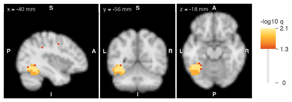
Orthogonal views through the left planted sphere with FDR-significant searchlight centres in orange-yellow, covering most of the sphere and a few voxels just outside it

Centres with FDR q < 0.05, coloured by −log10 q, through the left planted sphere. Significant centres just outside the sphere are expected, because their 8 mm searchlights include signal voxels.

# Null distribution from searchlights refitted with the
# labels shuffled within runs, pooled within five
# quantile bins of sphere size; FDR across the map
perm <- run_permutation_searchlight(
  smod, observed = sl, radius = 8,
  perm_ctrl = permutation_control(n_perm = 20,
                                  subsample = 0.05,
                                  seed = 1))

# p_adj_map is NA outside the mask; show centres with q < .05
logq <- -log10(perm$p_adj_map)

at  <- coord_to_grid(sp, centres[1, , drop = FALSE])
fig <- plot_ortho(mni, coord = at, overlay = logq,
                  ov_thresh = -log10(0.05),
                  cbar_title = "-log10 q",
                  crosshair = FALSE, label_size = 3.5)

Representational similarity analysis

rsa_design() takes one or more model RDMs, and its block_var argument removes pairs of patterns from the same run. rsa_model() computes the neural RDM in each region or sphere and compares it with the models by correlation or regression (regtype); with distmethod = "crossvalidated_euclidean" it replaces correlation distances with squared Euclidean distances estimated across independent partitions such as runs. rsa_neural_rdm() returns the neural RDM itself for inspection.

Excluding same-run pairs leaves 4,224 of the 4,560 pattern pairs. With both model RDMs in one regression, the part of each model not shared with the other correlates with the neural RDM at 0.20 for category and 0.06 for animacy (semipartial r).

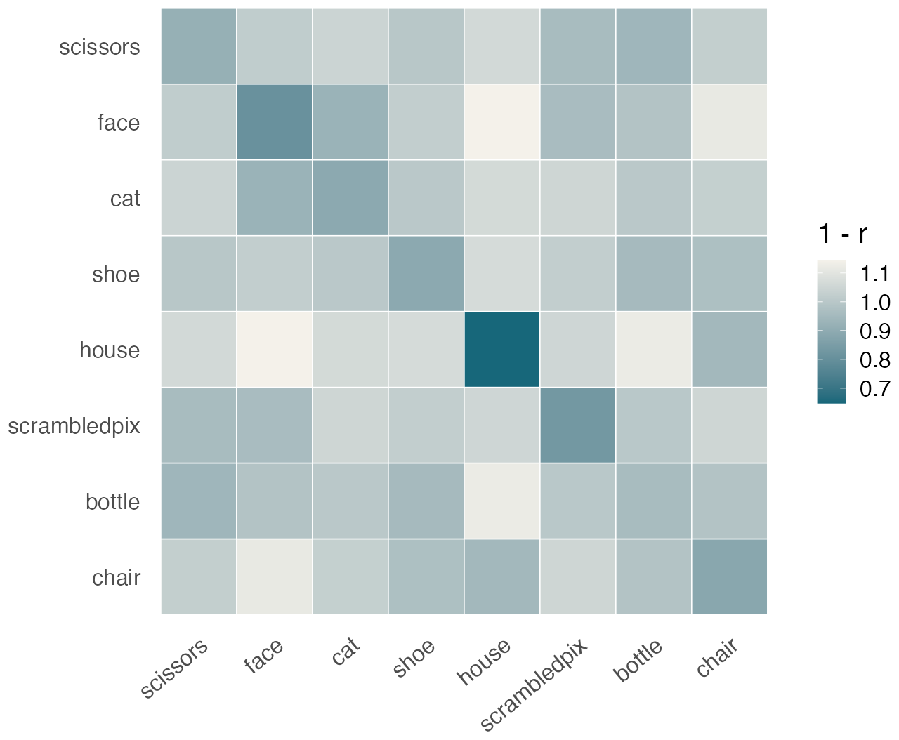
Eight-by-eight neural dissimilarity matrix for the Haxby categories; the lowest dissimilarity is between house patterns from different runs, the highest between house and face

Haxby et al. (2001), subject 1, after subtracting each run’s mean pattern. The matrix averages correlation distances over pairs from different runs, so the diagonal compares a category with itself across runs.

# RSA on the Haxby patterns. Subtract each run's mean
# pattern, then build two model RDMs (1 = different)
P <- hx$patterns
for (r in unique(hx$run)) {
  i <- hx$run == r
  P[i, ] <- scale(P[i, ], scale = FALSE)
}
anim     <- hx$category %in% c("face", "cat")
category <- outer(hx$category, hx$category, "!=") + 0
animacy  <- outer(anim, anim, "!=") + 0

# block_var drops pairs of patterns from the same run
rdes <- rsa_design(~ category + animacy,
                   list(category = category,
                        animacy = animacy),
                   block_var = hx$run)
cvec <- SparseNeuroVec(t(P), mask = vt,
                       space = add_dim(hx$mask_space, 96))
rmod <- rsa_model(mvpa_dataset(cvec, mask = vt), rdes,
                  distmethod = "pearson", regtype = "lm",
                  semipartial = TRUE)
rsa <- run_regional(rmod, region_mask = vt)
rsa$performance_table  # semipartial r per model RDM

# The neural RDM itself (1 - Pearson r), for display
D   <- rsa_neural_rdm(P, method = "pearson")
fig <- rdm_plot(D, hx$category, hx$run)

Built on

neuroim2 Image classes, masks and searchlight iterators

Every figure on this page is drawn by software/showcase/rMVPA/make-figures.R in the site’s source, and the code shown with each figure is the code that drew it. The simulation (simulate_bold()) and the two ggplot functions (confusion_plot(), rdm_plot()) are generic helpers in software/showcase/rMVPA/helpers.R.